0%

基于 PCA 的人脸识别方法--特征脸法[2]

基于 PCA 的人脸识别方法——特征脸法[2]

前言

这次主要说说 Matlab 实现与可视化。上次用了 YaleB 数据集不够好用,每个人的人脸图片数量不同,导致训练数据和测试数据划分比较麻烦。这次换了ORL数据集,好了些。

PCA

  1. 数据读取与预处理,ORL数据集一共400张图,40人,一个人10张。每个人10张照片,取4张作为测试数据,6张作为训练数据。
1
2
3
4
5
6
7
8
9
10
11
12
13
14
15
16
% 400张图,一共40人,一人10张
load('ORL4646.mat');

% 重塑后400列,一列是一张脸
reshaped_faces = reshape(ORL4646, 46*46,400);

% 取出前40%作为测试数据,剩下60%作为训练数据
test_data_index = [];
train_data_index = [];
for i=0:39
test_data_index = [test_data_index 10*i+1:10*i+4];
train_data_index = [train_data_index 10*i+5:10*(i+1)];
end

test_data = reshaped_faces(:, test_data_index);
train_data = reshaped_faces(:, train_data_index);

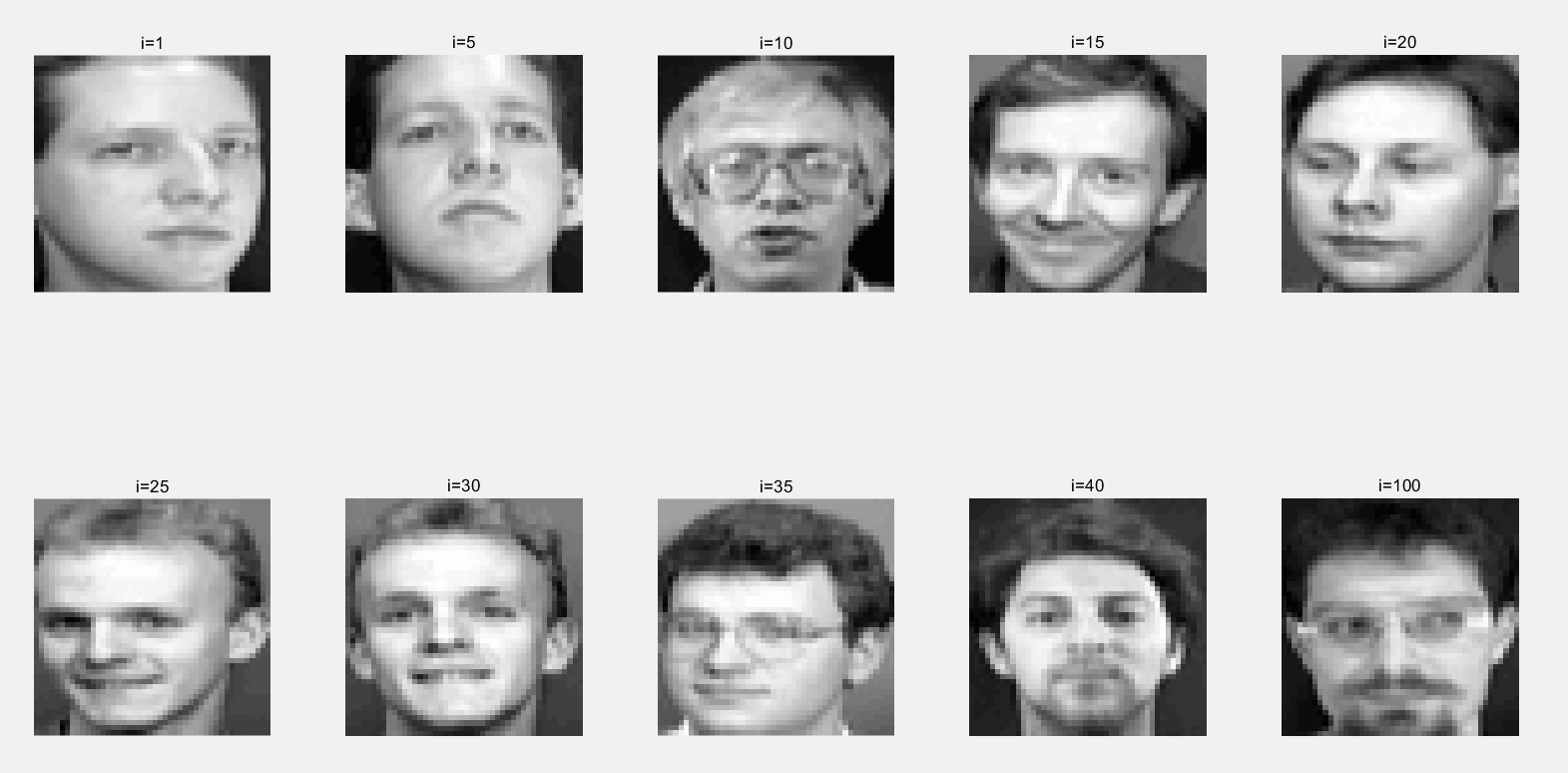
得到的训练数据和测试数据都是一个矩阵,每一列就是一张脸。通过提取训练数据中的部分列向量,重塑为方阵,并转化为灰度图像得到下图,代表了未经处理的原始数据,如图所示:

原始数据
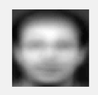
  1. 对训练数据的所有列向量求平均,得到平均列向量,将其重塑为图像即为”平均脸“,如图所示。由于该图像源于所有人脸的平均,所以直观上看可以看出人脸的轮廓,但五官细节较为模糊。

    1
    2
    % 求平均脸,即每一列分别求均值
    mean_face = mean(train_data, 2);
平均脸
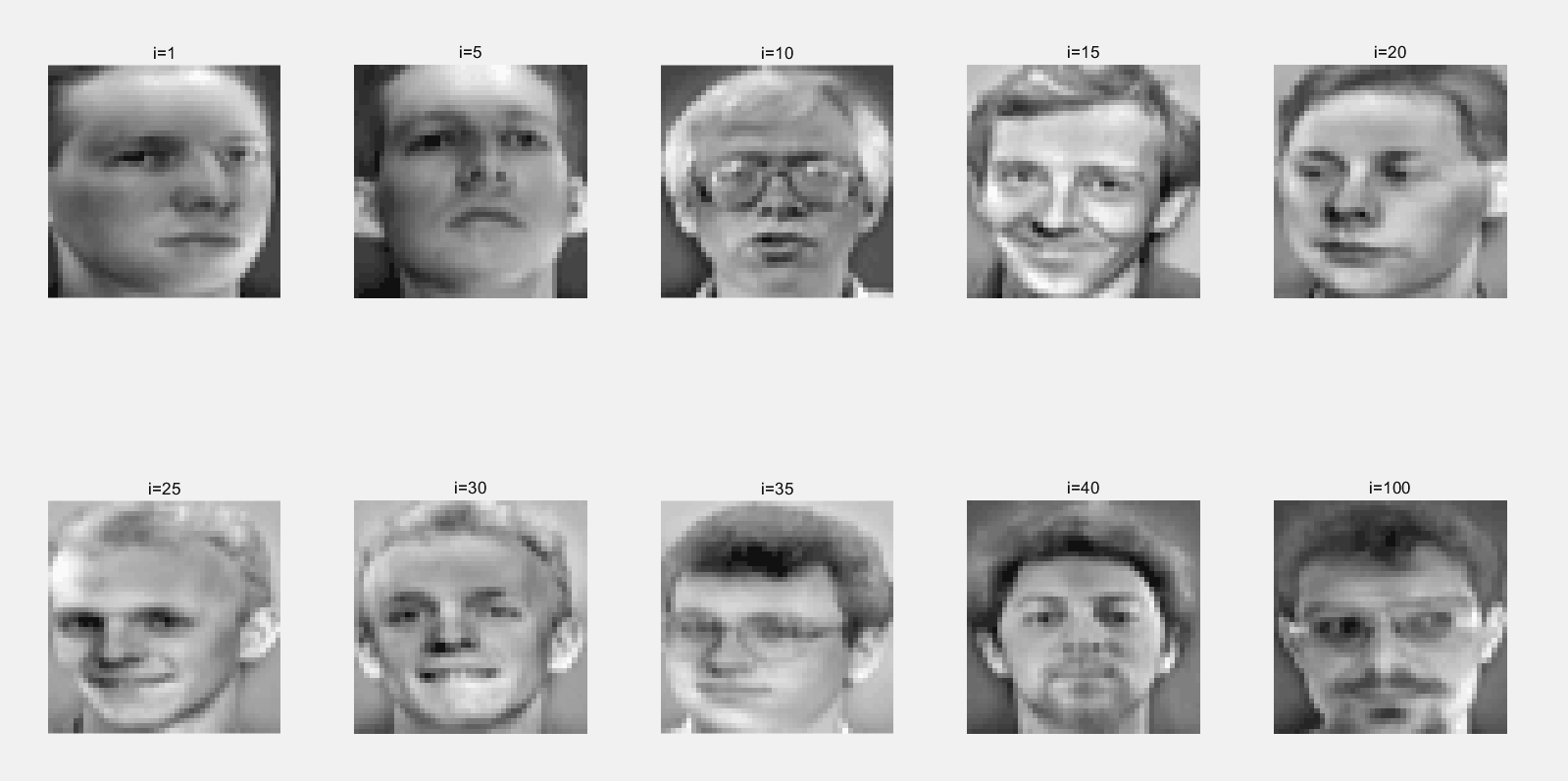
  1. 将所有列向量减去平均列向量,得到中心化后的数据。将部分中心化后的列向量重塑后转化为灰度图像,即为中心化后的脸。由于减去了平均人脸,因此相比原始人脸,中心化后的人脸的灰度值更低,图像直观上显得更加暗淡。

    1
    centered_face = (train_data - mean_face);
    中心化数据
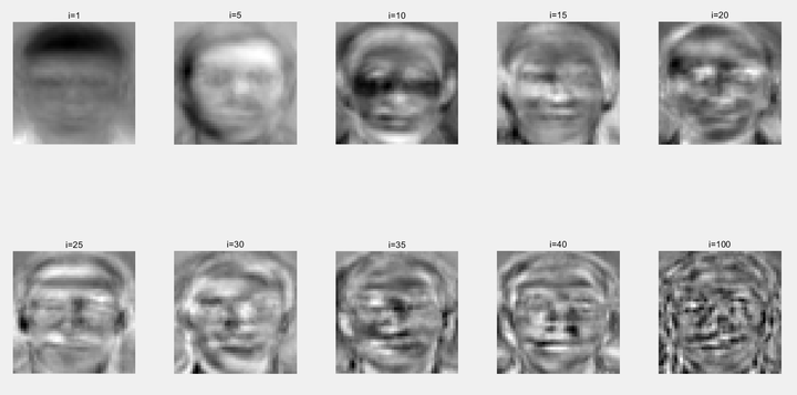
  2. 求出协方差矩阵的特征值与特征向量,将特征向量按照特征值大小排序。下图是部分特征向量通过重塑后转化为灰度图像得到的特征脸。从直观上可以看出随着特征值的降低,对应的特征脸越来越模糊,这是因为特征值大的特征脸保留了更多的有效信息。

    1
    2
    3
    4
    5
    6
    7
    8
    9
    10
    11
    12
    13
    14
    15
    % 协方差矩阵
    cov_matrix = centered_face * centered_face';
    [eigen_vectors, dianogol_matrix] = eig(cov_matrix);

    % 从对角矩阵获取特征值
    eigen_values = diag(dianogol_matrix);

    % 对特征值进行排序,获得排列后的特征值和索引
    [sorted_eigen_values, index] = sort(eigen_values, 'descend');

    % 获取排序后的征值对应的特征向量
    sorted_eigen_vectors = eigen_vectors(:, index);

    % 特征脸(所有)
    all_eigen_faces = sorted_eigen_vectors;

特征脸

值得一提的是,这里也可以使用SVD的方式去求特征脸,详见上文。

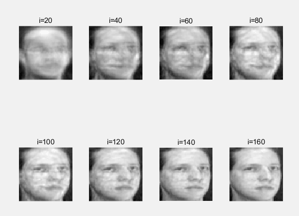
  1. 取出第一张人脸,使用不同数量的特征向量进行重构。
1
2
3
4
5
6
7
8
9
10
11
12
13
14
15
16
17
18
19
20
% 取出第一个人的人脸,用于重建
single_face = centered_face(:,1);

index = 1;
for i=20:20:160

% 取出相应数量特征脸
eigen_faces = all_eigen_faces(:,1:i);

% 重建人脸并显示
rebuild_faces = eigen_faces * (eigen_faces' * single_face) + mean_face;
subplot(2, 4, index);
index = index + 1;
fig = show_face(rebuild_faces);
title(sprintf("i=%d", i));

if (i == 160)
waitfor(fig);
end
end

下图是分别在20,40,60,…,160数量的特征向量下重构的人脸。从直观上可以看出随着特征向量数量的增加,重构出的人脸越来越清晰。这是因为使用越多的特征向量进行人脸重构,丢失的信息越少,因此重构出的人脸更加清晰。

使用不同的人脸进行重构

  1. 计算不同数量特征向量下,人脸的识别准确度,思路是:将人脸投影到低维空间中,计算未知人脸与所有已知人脸的距离(欧几里得距离),然后使用最近邻分类器KNN进行识别。最终的准确率在 93%-97% 之间。

    1
    2
    3
    4
    5
    6
    7
    8
    9
    10
    11
    12
    13
    14
    15
    16
    17
    18
    19
    20
    21
    22
    23
    24
    25
    26
    27
    28
    29
    30
    31
    32
    33
    34
    35
    36
    37
    38
    39
    40
    41
    42
    43
    44
    45
    46
    47
    48
    49
    50
    51
    52
    53
    54
    55
    56
    57
    58
    59
    60
    61
    62
    63
    64
    65
    66
    67
    68
    69
    70
    71
    72
    73
    74
    75
    76
    77
    78
    79
    80
    index = 1;
    X = [];
    Y = [];
    for i=10:10:160

    % 取出相应数量特征脸
    eigen_faces = all_eigen_faces(:,1:i);

    % 测试、训练数据降维
    projected_train_data = eigen_faces' * (train_data - mean_face);
    projected_test_data = eigen_faces' * (test_data - mean_face);

    % 开始测试识别率
    %%%%%%%%%%%%%%%%%%%%%%%%%%%%%%%%%%%%%%%%%%%%%%%%%

    % KNN的k值
    for k=1:6

    % 用于保存最小的k个值的矩阵
    % 用于保存最小k个值对应的人标签的矩阵
    minimun_k_values = zeros(k,1);
    label_of_minimun_k_values = zeros(k,1);

    % 测试脸的数量
    test_face_number = size(projected_test_data, 2);

    % 识别正确数量
    correct_predict_number = 0;

    % 遍历每一个待测试人脸
    for each_test_face_index = 1:test_face_number

    each_test_face = projected_test_data(:,each_test_face_index);

    % 先把k个值填满,避免在迭代中反复判断
    for each_train_face_index = 1:k
    minimun_k_values(each_train_face_index,1) = norm(each_test_face - projected_train_data(:,each_train_face_index));
    label_of_minimun_k_values(each_train_face_index,1) = floor((train_data_index(1,each_train_face_index) - 1) / 10) + 1;
    end

    % 找出k个值中最大值及其下标
    [max_value, index_of_max_value] = max(minimun_k_values);

    % 计算与剩余每一个已知人脸的距离
    for each_train_face_index = k+1:size(projected_train_data,2)

    % 计算距离
    distance = norm(each_test_face - projected_train_data(:,each_train_face_index));

    % 遇到更小的距离就更新距离和标签
    if (distance < max_value)
    minimun_k_values(index_of_max_value,1) = distance;
    label_of_minimun_k_values(index_of_max_value,1) = floor((train_data_index(1,each_train_face_index) - 1) / 10) + 1;
    [max_value, index_of_max_value] = max(minimun_k_values);
    end
    end

    % 最终得到距离最小的k个值以及对应的标签
    % 取出出现次数最多的值,为预测的人脸标签
    predict_label = mode(label_of_minimun_k_values);
    real_label = floor((test_data_index(1,each_test_face_index) - 1) / 10)+1;

    if (predict_label == real_label)
    %fprintf("预测值:%d,实际值:%d,正确\n",predict_label,real_label);
    correct_predict_number = correct_predict_number + 1;
    else
    %fprintf("预测值:%d,实际值:%d,错误\n",predict_label,real_label);
    end
    end

    correct_rate = correct_predict_number/test_face_number;

    X = [X k];
    Y = [Y correct_rate];

    fprintf("k=%d,i=%d,总测试样本:%d,正确数:%d,正确率:%1f\n", k, i,test_face_number,correct_predict_number,correct_rate);
    end
    end

    waitfor(plot(X,Y));
  2. 人脸投影到低维空间的可视化:分别将人脸投影到二维空间与三维空间,并画图。

1
2
3
4
5
6
7
8
9
10
11
12
13
14
15
16
17
18
19
20
21
22
% 二三维可视化
for i=[2 3]

% 取出相应数量特征脸
eigen_faces = all_eigen_faces(:,1:i);

% 投影
projected_test_data = eigen_faces' * (test_data - mean_face);

color = [];
for j=1:160
color = [color floor((j-1)/4)*5];
end

% 显示
if (i == 2)
waitfor(scatter(projected_test_data(1, :), projected_test_data(2, :), [], color));
else
waitfor(scatter3(projected_test_data(1, :), projected_test_data(2, :), projected_test_data(3, :), [], color));
end

end

效果:

二维投影

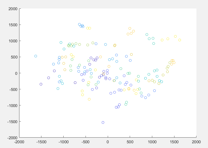
上图将人脸投影到二维空间下的可视化表示,每一个点代表一张人脸的图像,颜色相同的点代表同一个人的脸。

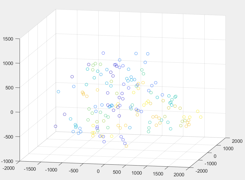
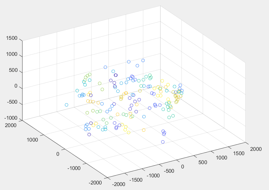
下面两图分别是在不同的两个角度下观察人脸数据在三维空间下的投影。其中每个点代表一张人脸图片,颜色相同的点代表同一人脸。由于同一人的人脸相近,因此颜色相同的点总是聚集地更加紧凑一些。

三维投影--角度一 三维空间--角度2

所有代码

1
2
3
4
5
6
7
8
9
10
11
12
13
14
15
16
17
18
19
20
21
22
23
24
25
26
27
28
29
30
31
32
33
34
35
36
37
38
39
40
41
42
43
44
45
46
47
48
49
50
51
52
53
54
55
56
57
58
59
60
61
62
63
64
65
66
67
68
69
70
71
72
73
74
75
76
77
78
79
80
81
82
83
84
85
86
87
88
89
90
91
92
93
94
95
96
97
98
99
100
101
102
103
104
105
106
107
108
109
110
111
112
113
114
115
116
117
118
119
120
121
122
123
124
125
126
127
128
129
130
131
132
133
134
135
136
137
138
139
140
141
142
143
144
145
146
147
148
149
150
151
152
153
154
155
156
157
158
159
160
161
162
163
164
165
166
167
168
169
170
171
172
173
174
175
176
177
178
179
180
181
182
183
184
185
186
187
188
189
190
191
192
193
194
195
196
197
198
199
200
201
clear all;

% 400张图,一共40人,一人10张
load('ORL4646.mat');

% 训练数据与测试数据的生成
%%%%%%%%%%%%%%%%%%%%%%%%%%%%%%%%%%%%%%%%%%%%%%%

% 重塑后400列,一列是一张脸
reshaped_faces = reshape(ORL4646, 46*46,400);

% 取出前40%作为测试数据,剩下60%作为训练数据
test_data_index = [];
train_data_index = [];
for i=0:39
test_data_index = [test_data_index 10*i+1:10*i+4];
train_data_index = [train_data_index 10*i+5:10*(i+1)];
end

test_data = reshaped_faces(:, test_data_index);
train_data = reshaped_faces(:,train_data_index);

waitfor(show_faces(train_data));

% 取得中心化数据
%%%%%%%%%%%%%%%%%%%%%%%%%%%%%%%%%%%%%%%%%%%%%%%

% 求平均脸,即每一列分别求均值
mean_face = mean(train_data, 2);
waitfor(show_face(mean_face));

% 中心化每一列是一个一张图
centered_face = (train_data - mean_face);
waitfor(show_faces(centered_face));

% 求得协方差矩阵的特征值与特征向量
%%%%%%%%%%%%%%%%%%%%%%%%%%%%%%%%%%%%%%%%%%%%%%%

% % 求内积矩阵,是协方差矩阵的替代
% % 内积矩阵的特征向量与对角矩阵
% inner_product_matrix = centered_face' * centered_face;
% [eigen_vectors, dianogol_matrix] = eig(inner_product_matrix);
% eigen_vectors = centered_face * eigen_vectors;

% 协方差矩阵
cov_matrix = centered_face * centered_face';
[eigen_vectors, dianogol_matrix] = eig(cov_matrix);

% 从对角矩阵获取特征值
eigen_values = diag(dianogol_matrix);

% 对特征值进行排序,获得排列后的特征值和索引
[sorted_eigen_values, index] = sort(eigen_values, 'descend');

% 获取排序后的征值对应的特征向量
sorted_eigen_vectors = eigen_vectors(:, index);

% 筛选出特征脸
%%%%%%%%%%%%%%%%%%%%%%%%%%%%%%%%%%%%%%%%%%%%%%%

% 特征脸(所有)
all_eigen_faces = sorted_eigen_vectors;
waitfor(show_faces(all_eigen_faces));

% 取出第一个人的人脸,用于重建
single_face = centered_face(:,1);

index = 1;
X = [];
Y = [];
for i=10:10:160

% 取出相应数量特征脸
eigen_faces = all_eigen_faces(:,1:i);

% 重建人脸并显示
if (mod(i,20)==0)
rebuild_faces = eigen_faces * (eigen_faces' * single_face) + mean_face;
subplot(2, 4, index);
index = index + 1;
fig = show_face(rebuild_faces);
title(sprintf("i=%d", i));

if (i == 160)
waitfor(fig);
end
end

% 测试、训练数据降维
projected_train_data = eigen_faces' * (train_data - mean_face);
projected_test_data = eigen_faces' * (test_data - mean_face);

% 开始测试识别率
%%%%%%%%%%%%%%%%%%%%%%%%%%%%%%%%%%%%%%%%%%%%%%%%%

% KNN的k值
for k=1:6

% 用于保存最小的k个值的矩阵
% 用于保存最小k个值对应的人标签的矩阵
minimun_k_values = zeros(k,1);
label_of_minimun_k_values = zeros(k,1);

% 测试脸的数量
test_face_number = size(projected_test_data, 2);

% 识别正确数量
correct_predict_number = 0;

% 遍历每一个待测试人脸
for each_test_face_index = 1:test_face_number

each_test_face = projected_test_data(:,each_test_face_index);

% 先把k个值填满,避免在迭代中反复判断
for each_train_face_index = 1:k
minimun_k_values(each_train_face_index,1) = norm(each_test_face - projected_train_data(:,each_train_face_index));
label_of_minimun_k_values(each_train_face_index,1) = floor((train_data_index(1,each_train_face_index) - 1) / 10) + 1;
end

% 找出k个值中最大值及其下标
[max_value, index_of_max_value] = max(minimun_k_values);

% 计算与剩余每一个已知人脸的距离
for each_train_face_index = k+1:size(projected_train_data,2)

% 计算距离
distance = norm(each_test_face - projected_train_data(:,each_train_face_index));

% 遇到更小的距离就更新距离和标签
if (distance < max_value)
minimun_k_values(index_of_max_value,1) = distance;
label_of_minimun_k_values(index_of_max_value,1) = floor((train_data_index(1,each_train_face_index) - 1) / 10) + 1;
[max_value, index_of_max_value] = max(minimun_k_values);
end
end

% 最终得到距离最小的k个值以及对应的标签
% 取出出现次数最多的值,为预测的人脸标签
predict_label = mode(label_of_minimun_k_values);
real_label = floor((test_data_index(1,each_test_face_index) - 1) / 10)+1;

if (predict_label == real_label)
%fprintf("预测值:%d,实际值:%d,正确\n",predict_label,real_label);
correct_predict_number = correct_predict_number + 1;
else
%fprintf("预测值:%d,实际值:%d,错误\n",predict_label,real_label);
end
end

correct_rate = correct_predict_number/test_face_number;

X = [X k];
Y = [Y correct_rate];

fprintf("k=%d,i=%d,总测试样本:%d,正确数:%d,正确率:%1f\n", k, i,test_face_number,correct_predict_number,correct_rate);
end
end

waitfor(plot(X,Y));

% 二三维可视化
for i=[2 3]

% 取出相应数量特征脸
eigen_faces = all_eigen_faces(:,1:i);

% 投影
projected_test_data = eigen_faces' * (test_data - mean_face);

color = [];
for j=1:160
color = [color floor((j-1)/4)*5];
end

% 显示
if (i == 2)
waitfor(scatter(projected_test_data(1, :), projected_test_data(2, :), [], color));
else
waitfor(scatter3(projected_test_data(1, :), projected_test_data(2, :), projected_test_data(3, :), [], color));
end

end


% 输入向量,显示脸
function fig = show_face(vector)
fig = imshow(mat2gray(reshape(vector, [46, 46])));
end

% 显示矩阵中某些脸
function fig = show_faces(eigen_vectors)
count = 1;
index_of_image_to_show = [1,5,10,15,20,25,30,35,40,100];
for i=index_of_image_to_show
subplot(2,5,count);
fig = show_face(eigen_vectors(:, i));
title(sprintf("i=%d", i));
count = count + 1;
end
end

本文地址: https://www.chimaoshu.top/基于-PCA-的人脸识别方法-特征脸法-2/
版权声明:本博客所有文章除特别声明外,均采用 Apache License 2.0 许可协议,转载请注明出处。

Welcome to my other publishing channels